
Forecast Your Sales For Better Planning
The most significant benefit of Defog is that it downloads Amazon Sellers’ data to Google Sheets and automatically updates it. Sellers may then use the data to do many things, one of the most interesting being forecasting their future sales.
In this article, we will walk you through creating a simple table to forecast the next months of sales for total units ordered and total revenue. You may also use the principle illustrated in this post to create a forecast for next week’s or quarter’s sales. You will be creating a table like the one below:
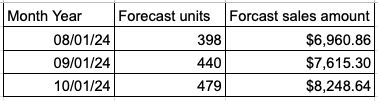
As soon as Defog updates the data, the forecast we will create below will be automatically updated. We will use Google Sheets’ forecast formula ().
Step 1: On your desktop browser, open your Defog spreadsheet on the OrdersTable tab.
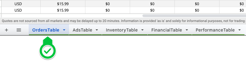
Image 1 – Open Defog on the OrdersTable tab
Step 2: Start by selecting the initial column of your pivot table. Click on the Column E.

Image 2 – Click column E
Step 3: Now select the final column of your pivot table. Shift-click on Column AC. You have selected all rows between Column E and AC, including the ones that will be added in future updates to the OrdersTable.
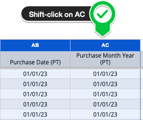
Image 3 – Shift-click column AC
Number of units and sales amount per month
Step 4: With the table selected in the previous steps, click Insert on the top Google Sheets menu and then click Pivot table (image 4.1). Then click Create in the pop-up window (Image 4.2). You will create a new tab on your Defog that will look like Image 4.3 below.
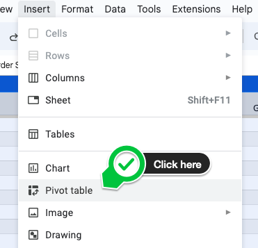
Image 4.1 – Click Insert > Pivot table
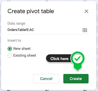
Image 4.2 – Create a pivot table on a new sheet
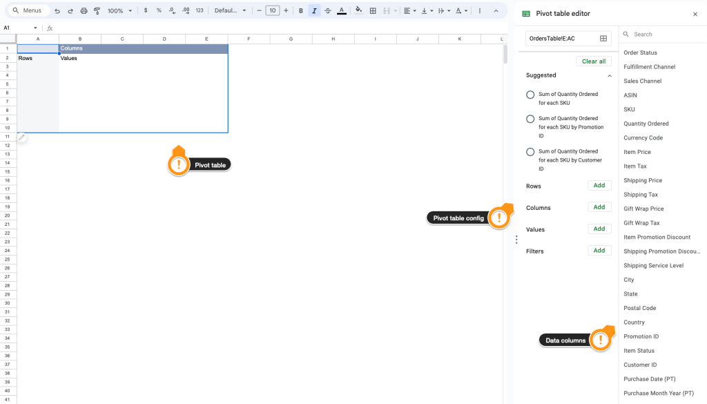
Image 4.3 – Your new pivot table
Step 5: Now is the time to populate your pivot table with the desired data. Let’s start by selecting the date period. First, click Purchase Month Year (PT) on the data columns to the right of the tab.

Image 5 – Click on Purchase Month Year (PT)
Step 6: Drag and drop the Purchase Month Year (PT) column to the area below the session Rows on the pivot table configuration column (image 6). On the new Purchase Month Year (PT) box, unselect the option Show totals and select Descending on the Order pulldown menu. All months with data will appear in descending order rows on your pivot table.
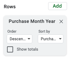
Image 6 – Purchase Month Year (PT) under Rows.
Step 7: Now, to select the pivot table values, let’s use the exact drag-and-drop mechanics above. Drop the Quantity Ordered and Item Price (the sales amount) below Values.
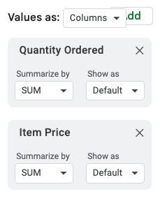
Image 7 – Quantity Ordered and Item Price on Values
Step 8: We must ensure that we only have closed months in our table to avoid using incomplete data from the current month on the forecast calculation. When we created this post, the current month was August 2024, so we will filter out 08/01/24 from our table. Drag and drop the Purchase Month Year (PT) column below the session Filters on the pivot table configuration column to do that. Next, on the Purchase Month Year (PT) box on Filters, click on Filter by condition and then on Custom formula is (the last option at the bottom of the menu). Copy and paste the following formula on the blank text box and click OK. The 08/01/24 line should disappear from the table.
='Purchase Month Year (PT)'<date(year(today()),month(today()),1)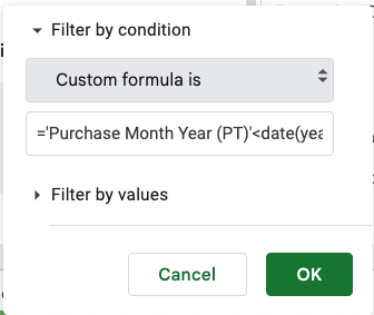
Image 8.1 – Purchase Month Year (PT) box on the Filters session
After a few cosmetic adjustments, the table looks like the image below.
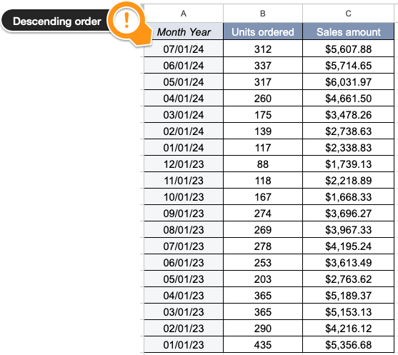
Image 8.2 – Base table for the forecasting
The forecast
You have completed your pivot table with the data for the forecasting. We will provide the forecast formula with the last six months of data and forecast the next three months. You may provide as many periods as you want or need.
Step 9: On the right side of your table, a couple of columns after it, create a new table like the one below, and supply it with the next three months. In this case, August, September, and October 2024.
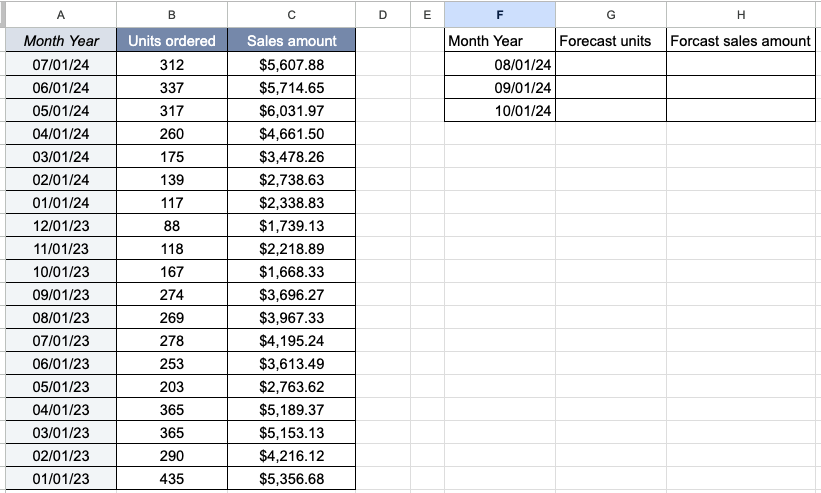
Image 9 – Base table and blank forecast table
Step 10: Add the formula below to cell G2 and copy it down to cell G4.
=round(forecast(F2,$B$2:$B$5,$A$2:$A$5))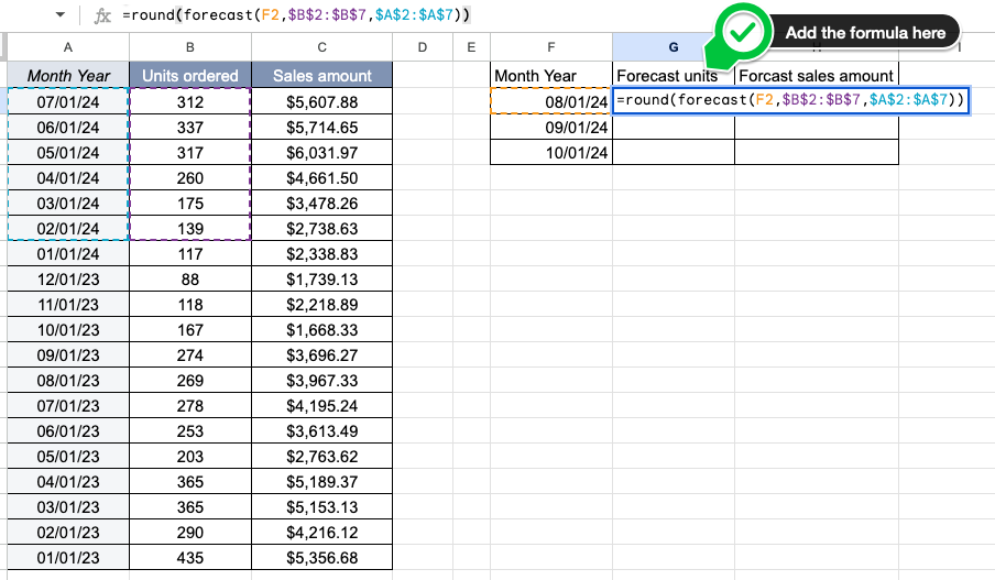
Image 10.1 – Adding the formula to forecast total units ordered
Then, add the formula below to cell H2 and copy it down to cell H4.
=forecast(F2,$C$2:$C$5,$A$2:$A$5)After a few other cosmetic adjustments, your forecast is ready and looks like Image 10.2 below.

Image 10.2 – 3-Months forecast
Please note that if you sell in more than one country in the same Amazon Region (North America, Europe, or Far East), Defog will download data from all countries (all marketplaces) to the same OrdersTable. You must do the forecast per country or currency, as you cannot sum the total sales amount in different currencies.
Now that you have learned how to use Defog and the forecast formula for the total quantity and sales amount, what about doing the same per SKU? It is certainly a good exercise! But there is a post for that.
If you want to learn what a particular column stands for on Defog’s tables, please visit our glossary.
Thank you for reading this post. If you still haven’t used Defog, use it for free here.
If you need any help, we are here for you.
Disclaimer: Defog is not responsible for any decisions made by the reader of this post regarding forecasting or any other use of the data and formulas provided.