Few things are more important for an Amazon seller than having products available for sale on Amazon’s virtual shelves. When you run out of stock, Amazon punishes your store, reducing your exposure.
The metrics you need to forecast your store’s remaining days of inventory for a particular SKU are its sales velocity and the number of units available for sale, whether you sell through FBA or FBM.
Calculate Sales Velocity per SKU for Amazon Sellers
The most significant benefit of Defog is that it integrates Amazon Seller Central’s data with Google Sheets, automatically updating the data. Sellers may then use the data to control their inventory and forecast the remaining days of stock they have.
The remaining inventory in days and the lead time (the time it takes to receive new inventory from your suppliers) are then used to buy new inventory at the right time and in the right amounts.
In this article, we will show you how to calculate the sales velocity per SKU by creating a simple table with each SKU’s number of units sold in three different periods: the last seven days, 14 days, and 28 days. You may use the same mechanics for other periods, say eight weeks. Also, if you want to forecast special events like Amazon Prime Day or Black Friday, having last year’s data, you can calculate the sales velocity for the same period the previous year, including the special event, to forecast what will happen this year.
You will be creating a table like the one below:
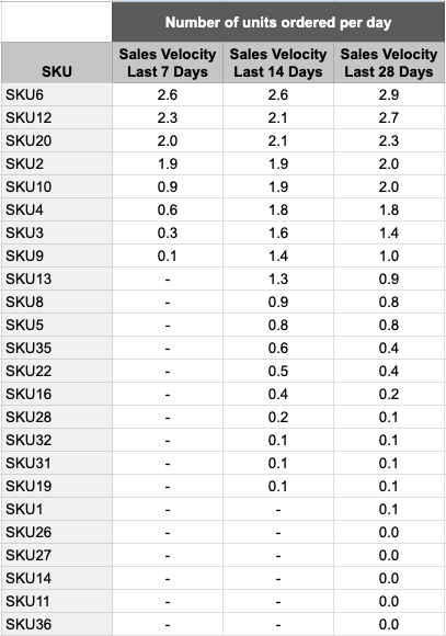
One good thing about doing this in Defog’s spreadsheet is that the table above will automatically update with new orders as soon as Defog updates.
Step 1: On your desktop browser, open your Defog spreadsheet on the OrdersTable tab.
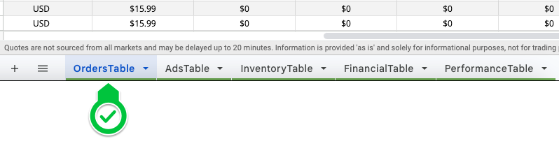
Image 1 – Open Defog on the OrdersTable tab
Step 2: Start by selecting the initial column of your pivot table. Click on the Column E.
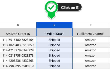
Image 2 – Click column E
Step 3: Now select the final column of your pivot table. Shift-click on Column AC. You have selected all rows between Column E and AC, including the ones that will be added in future updates to the OrdersTable.
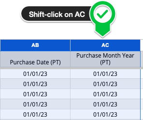
Image 3 – Shift-click column AC
Total number of orders per SKU per period
Step 4: With the table selected in the previous steps, click Insert on the top Google Sheets menu and then click Pivot table (image 4.1). Then click Create in the pop-up window (Image 4.2). You will create a new tab on your Defog that will look like Image 4.3 below.
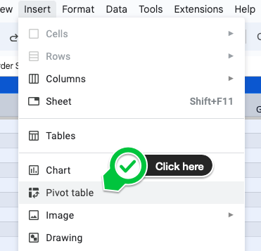
Image 4.1 – Click Insert > Pivot table
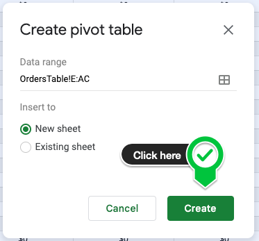
Image 4.2 – Create a pivot table on a new sheet
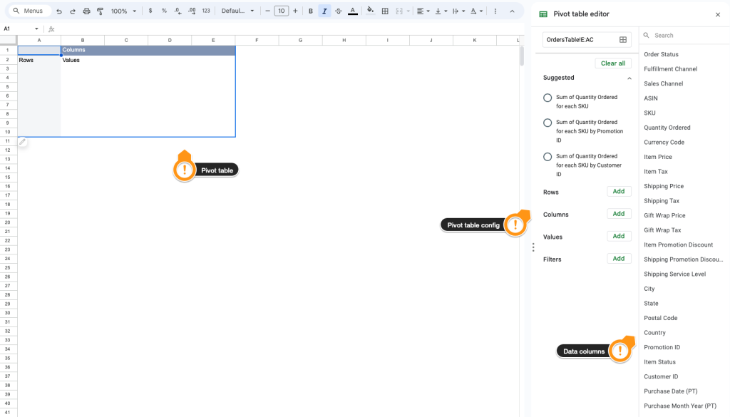
Image 4.3 – Your new pivot table
Step 5: Now is the time to populate your pivot table with the desired data. Let’s start by selecting the SKU. First, click SKU on the data columns to the right of the tab.

Image 5 – Click on SKU
Step 6: Drag and drop the SKU column to the area below the session Rows on the pivot table configuration column (image 6.1). On the new SKU box, unselect the option Show totals. All SKUs will appear in the first column on your pivot table.
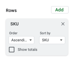
Image 6.1 – SKU under Rows
Step 7: Use the drag-and-drop mechanics above to select the pivot table values. Drag the Quantity Ordered data column below Values (Image 7.1). Then, return to the SKU box under Rows and change the Order pulldown-menu to Descending and Sort by to SUM of Quantity Ordered (Image 7.2).

Image 7.1 – Quantity Ordered in Values session
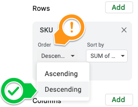
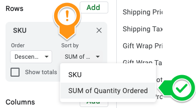
Image 7.2 – Set the two pull-down menus on the SKU box
Step 8: Let’s set the period for the last 7 days. To be precise, our calculation is from the 8th day before today up to yesterday, as we must ensure that we filter out the current day as it is not finished yet. To do that, drag and drop the Purchase Date (PT) data column below the session Filters on the pivot table configuration column. Next, on the Purchase Date (PT) box on Filters, click on Status > Filter by condition and then on Custom formula is (the last option at the bottom of the menu). In the blank text box, copy and paste the following formula and click OK (Image 8.1).
=AND('Purchase Date (PT)' >= date(year(today()),month(today()),day(today())-8), 'Purchase Date (PT)' < today())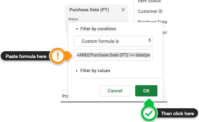
Image 8.1 – Purchase Date filter
After a few cosmetic adjustments, the table looks like the image below.
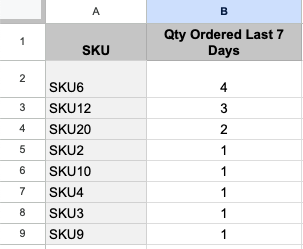
Image 8.2 – Quantity Ordered Last 7 Days
Step 9: Copy the pivot table to the space on its right side, giving one column of space between them, then change the custom formula on the Purchase Date (PT) box under Filters to:
=AND('Purchase Date (PT)' >= date(year(today()),month(today()),day(today())-15), 'Purchase Date (PT)' < today())Then do this again, copy the pivot table to the right and change the formula to:
=AND('Purchase Date (PT)' >= date(year(today()),month(today()),day(today())-29), 'Purchase Date (PT)' < today())In the end, you will have three separate pivot tables like in Image 9 below:
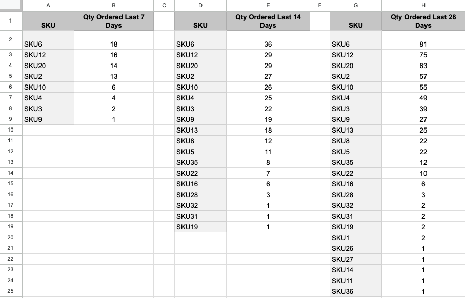
Image 9 – The three periods pivot table
Sales Velocity per Day per SKU
Step 10: To calculate the sales velocity per day, create a new table heading on the right of your pivot tables, as shown in Image 10.1 below.
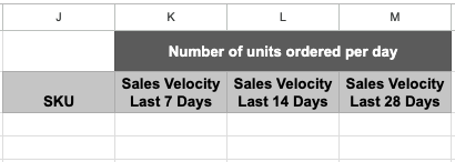
Image 10.1 – Headings for the Sales Velocity table
Copy and paste the following formulas into J3, K3, L3, and M3.
In J3: Unique SKUs with sales in the last 28 days
=filter(unique(flatten(A2:A,D2:D,G2:G)),unique(flatten(A2:A,D2:D,G2:G))<>"")In K3: Sales velocity per day in the last seven days
=iferror(arrayformula(if($J3:$J<>"",VLOOKUP($J3:$J,A:B,2,false)/7,"")),"-")In L3: Unique SKUs with sales in the last 17 days
=iferror(arrayformula(if($J3:$J<>"",VLOOKUP($J3:$J,D:E,2,false)/14,"")),"-")In M3: Sales velocity per day in the last 28 days
=iferror(arrayformula(if($J3:$J<>"",VLOOKUP($J3:$J,G:H,2,false)/28,"")),"-")Your Sales Velocity table will look like the one below.
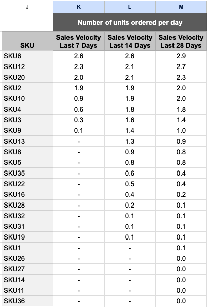
Image 10.2 – Base table with Orders from Repeat Customers
There are some things to highlight about this Sales Velocity table: first, it may not have all your store’s SKUs, as the pivot tables only present SKUs that had sales in the period included in the filter. Second, you see decimal numbers of units, but units should be whole numbers, right?! Well, the Sales Velocity per se is only part of the story. We need to divide the total inventory available by the sales velocity to calculate the number of days of inventory per SKU. So, let’s wait until we get to the remaining inventory days to round things.
What about calculating the number of remaining inventory days left by yourself? A hint: use Defog’s InventoryTable to determine the number of units available for sale, and then you are a division away.
If you want to learn what a particular column stands for on Defog’s tables, please visit our glossary.
Thank you for reading this post. If you still haven’t used Defog, you can do so for free here.
If you need any help, we are here for you.
Disclaimer: Defog is not responsible for any decisions made by the reader of this post or any other use of the data and formulas provided.