Sometimes, a store has too many products to monitor at once. If this is your case, your company has some sort of categorization by size, color, volume, or others. Keeping track of sales per category is a good business practice as you may make decisions based on a broader perspective. For example, you may decide that one category needs promotions or is not worth selling.
Monitor your sales, or any other figure, by product category
The most significant benefit of Defog is that it connects to Amazon Seller Central, automatically retrieving valuable data to Google Sheets. Sellers may then use the data to monitor how their products sell by category over time.
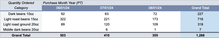
This article will show you how to create a table to calculate the units sold per category for the last three closed months. With minimal formula editing, you can apply the same principles to compare other metrics, such as sales amount, sales from advertising, number of refunded units, and more. You will create a table similar to the one below.
One significant advantage of using Defog’s spreadsheet is that whenever Defog updates the data, the table we create will automatically reflect those updates. Additionally, we will use today’s date as the base for the period, ensuring that the period is automatically recalculated every new month. The automatic updates enhance the efficiency and accuracy of your analysis, guaranteeing that you are making decisions with the most updated data.
Create product categories
Defog only downloads data from Amazon, and your company’s categories are unavailable on Amazon Seller Central. To create a category analysis, Defog needs to know your categories. Let’s start by creating a table to add each product’s category.
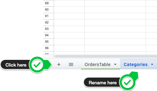
Step 1: On your desktop browser, open your spreadsheet. To create a new worksheet for the categories, click on the plus + symbol at the bottom left of the spreadsheet and change the new sheet name to Categories. The Categories sheet will have a table where you can add your products and their respective categories.
Create the Categories table
Step 2: In the Category sheet, use the UNIQUE formula to extract distinct values from the SKU column in the OrdersTable. This will ensure that the Category table gets automatically updated with new SKU entries as they are added to the OrdersTable. Copy and paste the formula below to the A1 cell on the new Categories sheet.
=UNIQUE(OrdersTable!I:I)Step 3: Next, you can use column B in the categories sheet to manually enter categories for each unique SKU. We usually paint cells with a blue background to remind us that someone should type in the values. The SKUs in column A will be automatically populated by the UNIQUE formula in Step 2 above, and column B will remain editable for you to assign your company’s categories, as in the example shown in the table below.
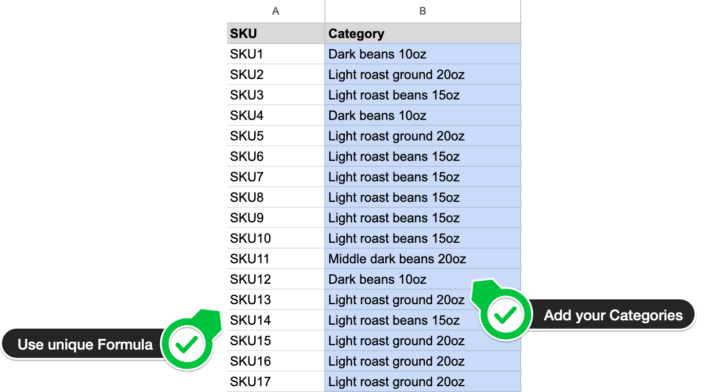
Add each SKU’s category.
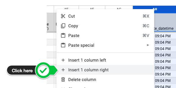
Step 4: Go to the OrdersTable and select the column AH. Click on the mouse button and click on + Insert 1 column right. Edit the title in the new column (AI) as Category.
Create a new column to add the order’s item category
This column will map the SKUs from the OrdersTable to their corresponding categories from the new Categories table.
Each row in the OrdersTable has an SKU. We will use a formula to look up the SKU’s category and add it to the new AI column. Copy and paste the formula below into cell AI2.
=ARRAYFORMULA(IF(I2:I<>"", VLOOKUP(I2:I, Categories!A:B, 2, FALSE), ""))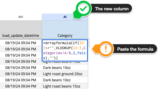
Insert the category lookup formula
Congrats, you did it! You now have a new column with each order’s category.
Summarize your sales per category
Step 5: In the OrdersTable, start by selecting the initial column of your pivot table. Click on Column I.
Click column I
Step 6: Now select the final column for your pivot table by shift-clicking on column AI. You have selected all rows between Column I (SKU) and the new Column AI (Category). This selection includes all the relevant data and ensures that any new entries added in future updates to the OrdersTable will also be included.
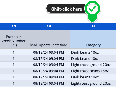
Shift-click column AL
Step 7: With the table selected in the previous steps, click Insert on the top Google Sheets menu and then click Pivot table (first image below). Then click Create in the pop-up window (second image). You will create a new tab on your Defog that will look like the third image.
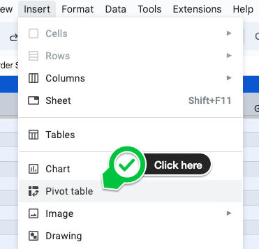
Click Insert > Pivot table
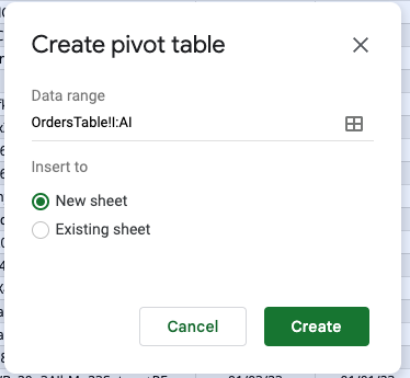
Create a pivot table on a new sheet
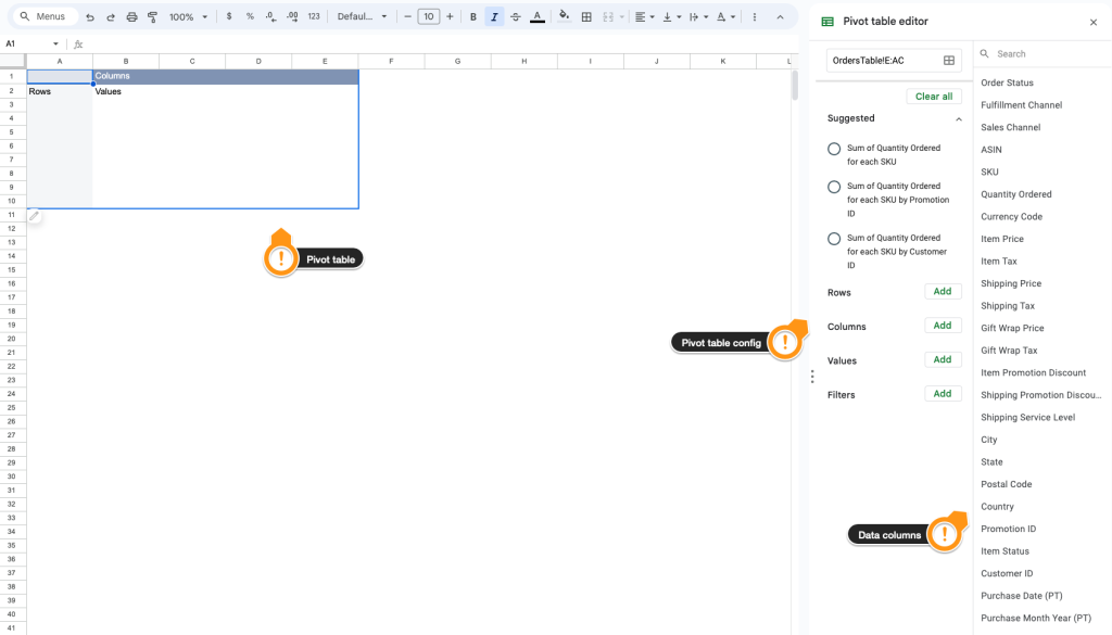
Your new pivot table
Step 8: Now, it’s time to populate your pivot table with the desired data. First, click Purchase Month Year (PT) in the data column on the right side of the pivot table tab.

Click on Purchase Month Year (PT)
Step 9: Drag and drop the Purchase Month Year (PT) column to the Columns section in the pivot table configuration panel. All the months will now appear in the first row of your pivot table.
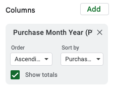
Purchase Month Year (PT) under Rows
Step 10: Drag and drop the Category column to the Rows section in the pivot table configuration panel. All the categories will now appear in the first column of your pivot table.
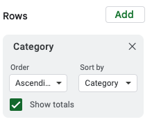
Category under Columns
Step 11: Use the drag-and-drop mechanics from earlier to configure your pivot table values. Drag the Quantity Ordered data column to the Values section.
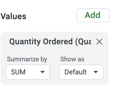
Quantity Ordered on Values
Step 12: To correctly filter the table and show only the last three closed months, you need to apply a filter to the Purchase Month Year (PT) row. Drag and drop the Purchase Month Year (PT) data column to the filters Filters section.
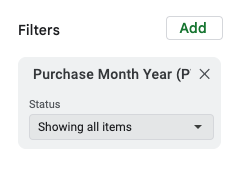
Posted Date box on the Filters section
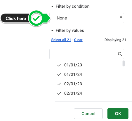
To filter in only the three previous closed months, we click on the Purchase Month Year (PT) Status pulldown, then click Filter by condition, and then choose Custom formula (the last option at the bottom).
Paste the formula below in the custom formula text box.
=AND('Purchase Month Year (PT)' >= date(year(today()),month(today())-3,1), 'Purchase Month Year (PT)'<date(year(today()),month(today()),1))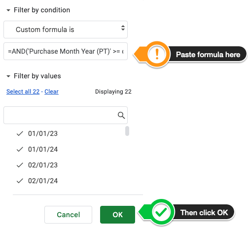
Poste the formula on the box in the Filters section
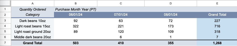
Step 13: Your final table looks like the image below after cosmetics editing.
Please note that if you sell in more than one country in the same Amazon Region (North America, Europe, or the Far East), Defog will download data from all countries (all marketplaces) to the same OrdersTable, and the data from different countries will be summed up on the table above.
If you want to learn what a particular column stands for on Defog’s tables, please visit our glossary.
Thank you for reading this post. If you still haven’t used Defog, you can do so for free here.
If you need any help, we are here for you.
Disclaimer: Defog is not responsible for any decisions made by the reader of this post or for the consequences of using the data, formulas, and charts provided.