Improve your products and listing to reduce refunds

Consumers regularly return products on Amazon, which impacts the sellers’ customer satisfaction indicators. Keeping track of what is being returned is a good business practice.

Amazon sellers may reduce the number of returns by changing the product’s description or pictures to help the consumer better understand what they are buying or even making changes to the product to increase its quality. 

Refunded orders

The most significant benefit of Defog is that it integrates with Amazon Seller Central, automatically retrieving and updating valuable data to Google Sheets. Sellers may then use the data to monitor their refunded orders per SKU and quickly spot products that need changes. 

In this article, we will create the tables below showing the number of units and the total amount returned for the current month and the last three months. You may use the same table to see other periods or to calculate the total refunded amount instead of per SKU.

One good thing about doing this in Defog’s spreadsheet is that the tables will be automatically updated as soon as Defog updates the data. Additionally, we will use today’s date as the base for the current month and the last three months; therefore, the current date and the previous period will be automatically recalculated every time the spreadsheet is opened.

Step 1:  On your desktop browser, open your Defog spreadsheet on the FinancialTable tab.

Open Defog on the FinancialTable tab

Step 2: Start by selecting the initial column of your pivot table. Click on the Column D.

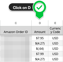
Click column D

Step 3: Now select the final column of your pivot table. Shift-click on Column L. You have selected all rows between Columns D and L, including the ones that will be added in future updates to the FinancialTable.

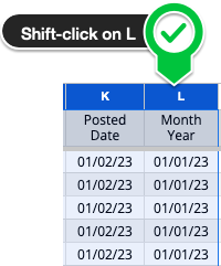
Shift-click column L

Number of units refunded per SKU

Step 4: With the table selected in the previous steps, click Insert on the top Google Sheets menu and then click Pivot table. Then click Create in the pop-up window. You will create a new tab on your Defog that will look like the image below.

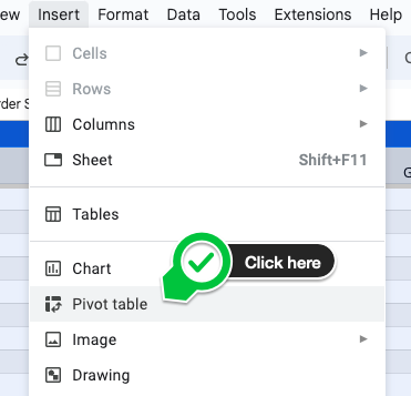
Click Insert > Pivot table

Create a pivot table on a new sheet

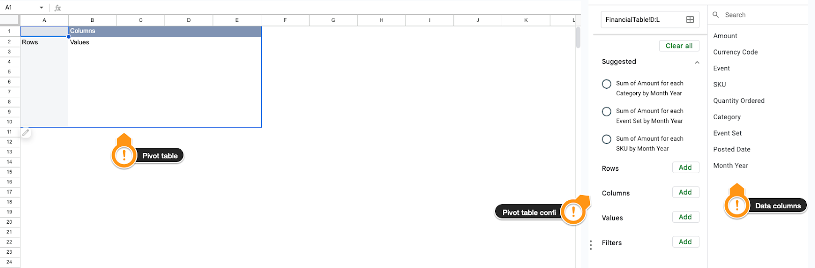
Your new pivot table

Step 5: Now is the time to populate your pivot table with the desired data. Let’s start by selecting the SKU. First, click SKU on the data columns to the right of the tab.

Click on SKU

Step 6: Drag and drop the SKU column to the area below the section Rows on the pivot table configuration column. All SKUs will appear in the first column on your pivot table.

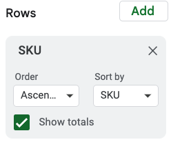
SKU under Rows

The tables we want to create will track refunds per month. To do that, we drag and drop the Month Year data column below the Columns section:

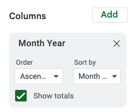
Month Year under Columns

Step 7: To select the first pivot table values, let’s use the exact drag-and-drop mechanics above. Drag Quantity Ordered below Values.

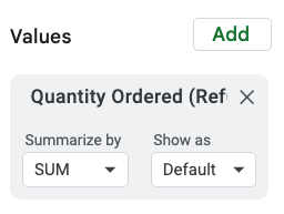
Quantity Ordered on Values

Step 8: To correctly filter the table and show only the refunded units, we must filter the Event column data to only Refund – Principal. Drag and drop the Event data column under Filters, then click on Status, then on the dropdown menu (image below), click on Clear, then on the text box, copy-and-paste Refund – Principal, click on the option in the list of values, and click OK to finish. 

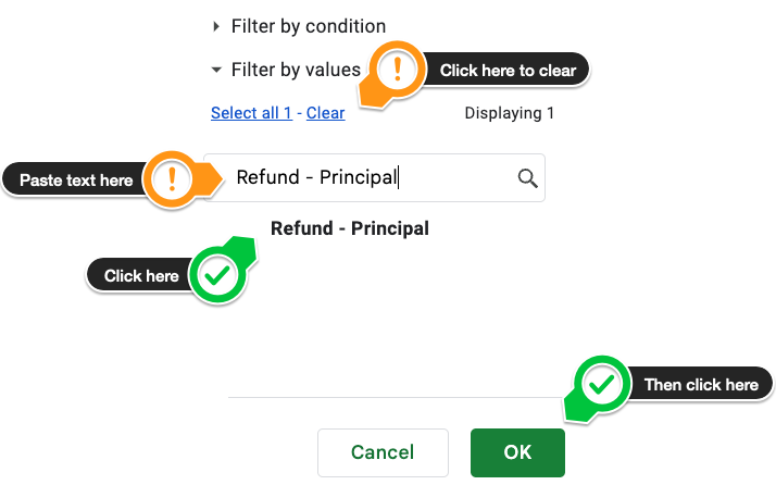
Filter Event to only show Refund – Principal

We must drag and drop the Posted Date column into the Filters section to show only the current month and the three previous months. Click on the Posted Date Showing all items pulldown menu, select Filter by condition, and then choose Custom formula (the last option at the bottom). Paste the formula below in the text box.

='Posted Date'>=date(year(today()),month(today())-3,1)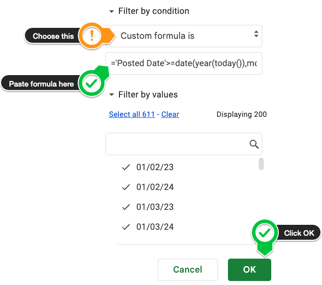

Posted Date box on the Filters section

Step 9: After a few cosmetic adjustments, the first table is ready and looks like the image below.

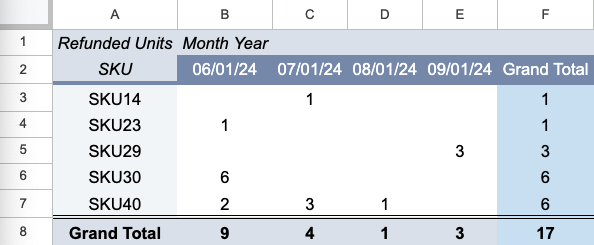
First Table – Refunded Units

Amount refunded per SKU

Step 10: To create the second table, we select the whole first table, copy and paste it to the right, let’s say into column H. Then we open the second pivot table settings by clicking on the pencil icon below it:

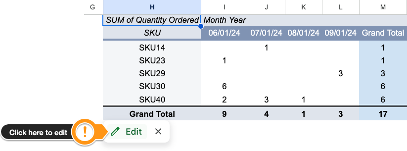
Edit the second table

In the second pivot table settings, we remove the Quantity Ordered box from the Values section (just click on the X at the box’s top right corner) and drag and drop the Amount data column to the Values section. 

You’re done! The two tables are ready. After some cosmetics editions, you have something like the tables below:

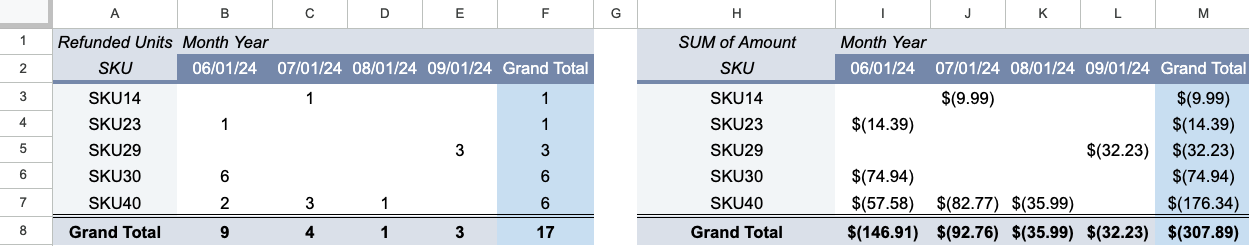
Please note that only refunded SKUs will be listed in the tables. 

You may change the tables’ period to show more or less months or remove the SKU from the rows section to show only the total refunded units and amounts.  

If you want to learn what a particular column stands for on Defog’s tables, please visit our glossary.

Thank you for reading this post. If you still haven’t used Defog, you can do so for free here.

If you need any help, we are here for you.

Disclaimer: Defog is not responsible for any decisions made by the reader of this post or for the consequences of using the data, formulas, and charts provided.