It is nice to know the total number of orders from repeat customers. However, to manage our product portfolio and pricing strategy and decide on Amazon programs like Subscribe & Save, it is important to know the percentage of orders from repeat customers per SKU.

Calculate the number of repeat customers’ orders per SKU

The most significant benefit of Defog is that it integrates Amazon Seller Central’s data with Google Sheets, automatically keeping the data current. Sellers may then use the data for their product portfolio management by calculating the percentage of orders from customers who bought a product more than once. 

In this article, we will show you how to calculate the percentage of orders from repeat customers per SKU by creating a simple table with each SKU’s total orders and orders from unique customers. Then, we will use this table to quickly calculate the percentage of orders from repeat customers per product.

You will be creating a table using conditional formatting like the one below:

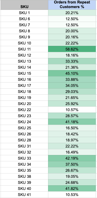
One advantage of doing this in Defog’s spreadsheet is that the table above will automatically update as soon as new orders arrive.

Let’s do this!

Step 1:  On your desktop browser, open your Defog spreadsheet on the OrdersTable tab.

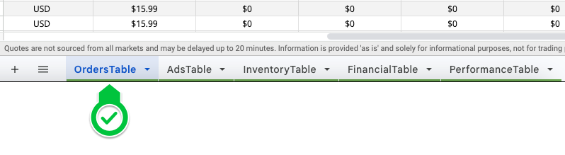
Image 1 – Open Defog on the OrdersTable tab

Step 2: Start by selecting the initial column of your pivot table. Click on the Column E.

Image 2 – Click column E

Step 3: Now select the final column of your pivot table. Shift-click on Column AC. You have selected all rows between Column E and AC, including the ones that will be added in future updates to the OrdersTable.

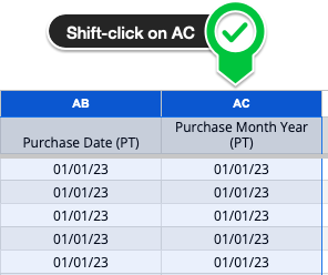
Image 3 – Shift-click column AC

Total number of orders per SKU

Step 4: With the table selected in the previous steps, click Insert on the top Google Sheets menu and then click Pivot table (image 4.1). Then click Create in the pop-up window (Image 4.2). You will create a new tab on your Defog that will look like Image 4.3 below.

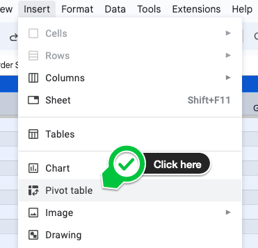
Image 4.1 – Click Insert > Pivot table

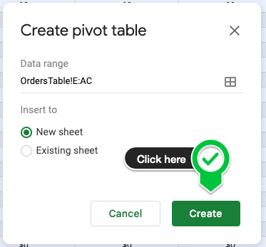
Image 4.2 – Create a pivot table on a new sheet

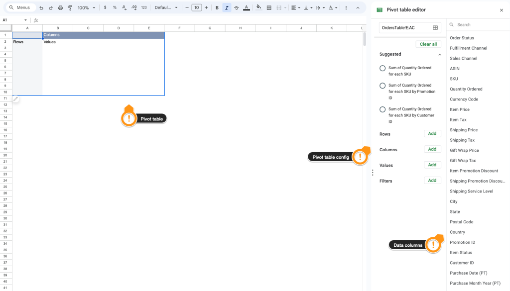
Image 4.3 – Your new pivot table

Step 5: Now is the time to populate your pivot table with the desired data. Let’s start by selecting the SKU data column. First, click SKU on the data columns to the right of the tab.

Image 5 – Click on SKU

Step 6: Drag and drop the SKU column to the area below the session Rows on the pivot table configuration column (image 6.1). On the new SKU box, unselect the option Show totals. All SKUs will appear in the first column on your pivot table.

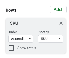
Image 6.1 – SKU under Rows

Step 7: Select the pivot table values from the drag-and-drop mechanics above. Drag the Customer ID data column below Values and then drag it again under Values (Image 7.1). The second time you drag Customer ID under Values, select COUNTUNIQUE from the Summarize by pull-down menu, as shown in Image 7.2.

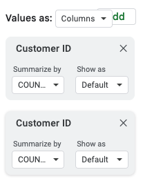
Image 7.1 – Customer ID dragged twice to the Values session

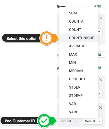
Image 7.2 – Customer ID summarized by COUNTUNIQUE

Step 8: After a few cosmetic adjustments, the table looks like the image below.

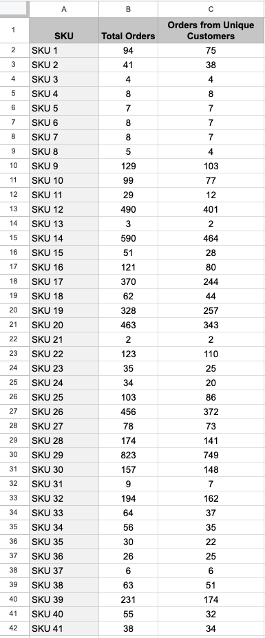
Image 8 – Base table: Customer orders per SKU

Number of orders from repeat customers calculation

Step 9: To get the percentage of orders from repeat customers, we must calculate the difference between Total Orders and Total Orders from Unique Customers. To do that, add two columns to the right of your pivot table, as shown in Image 9.1 below.

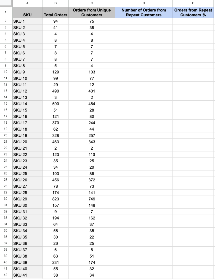
Image 9.1 – Add two new columns to the right of your pivot table

Now, copy and paste the following formulas into D2 and E2. 

In D2: Orders from Unique Customers minus Total Orders

=arrayformula(if(A2:A<>"",B2:B-C2:C,"")) 

In E2: Percentage of Total Orders that come from Repeat Customers

=arrayformula(if(A2:A<>"",if(B2:B>0,D2:D/B2:B,""),""))

Your table will look like the one below.

Image 9.2 – Base table with Orders from Repeat Customers

Step 10: The table above has some SKUs with few re-orders, so let’s make a new, cleaner, and more informative table by filtering out every SKU with less than 10% of orders from repeat customers. 

Add two columns to the right of your pivot table, like Image 10 below.

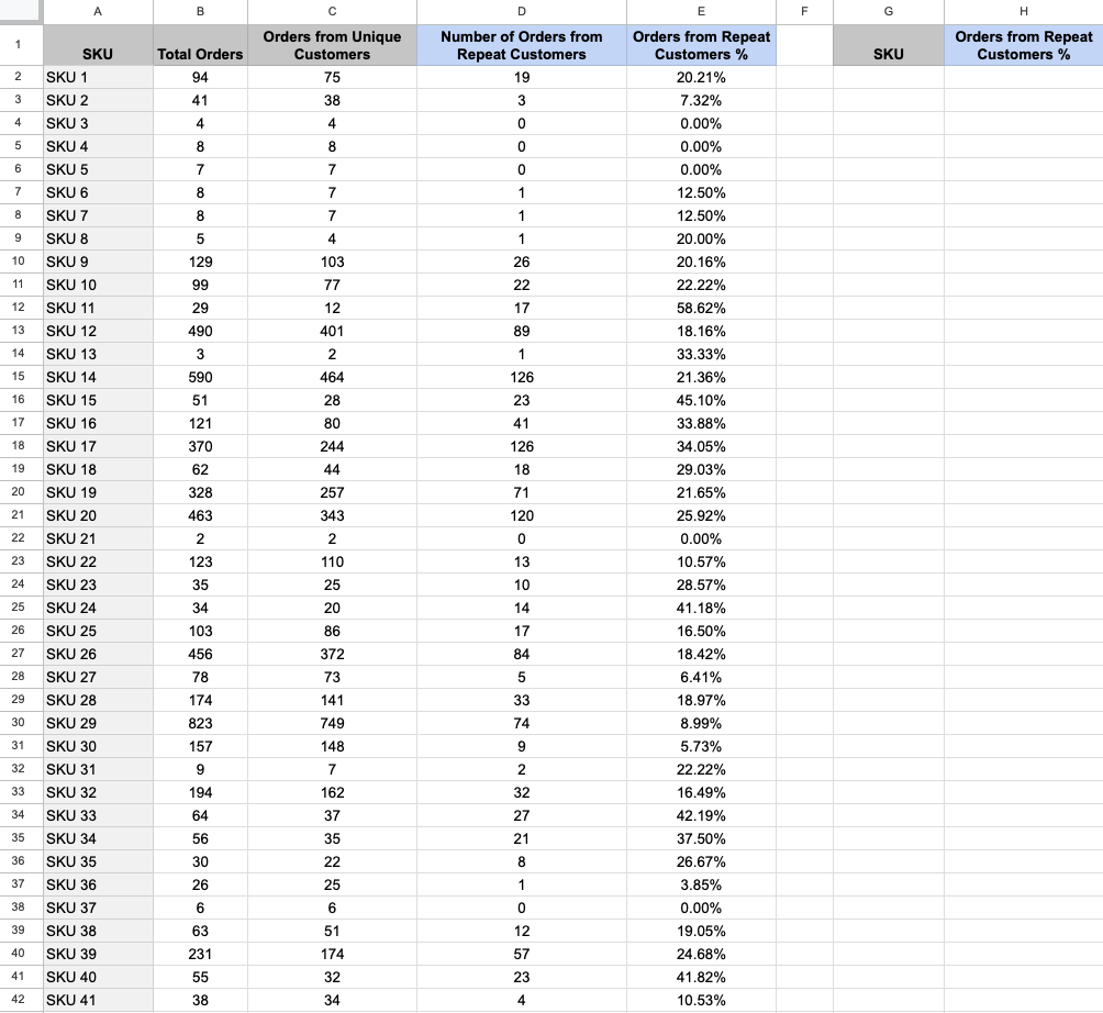
Image 10 – New table

Now, copy and paste the following formulas into G2 and H2. These formulas will filter out every SKU with less than 10% of orders from repeat customers so we can focus on those SKUs with more re-orders. 

In G2: FIlter the SKUs.

=filter(A2:A,E2:E>0.1)

In H2: Filter the percentages.

=filter(E2:E,E2:E>0.1)

Step 11: Now, let’s add the conditional formatting to the percentage column (H) so we can quickly see the SKUs on a scale from more orders from repeat customers to fewer. Click on column H. Then click Format > Conditional formatting.

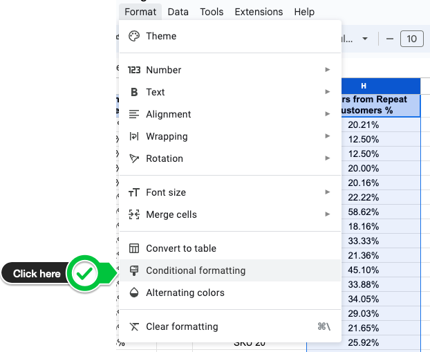
Image 11.1 – To open the Conditional formatting sidebar

Choose the Color scale as in Imagem 11.2, then click Done.

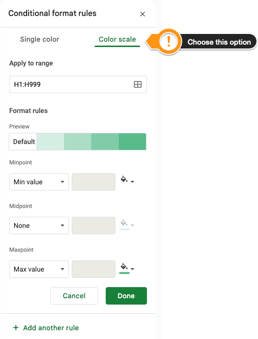
 11.2 – Color scale conditional formatting

Your table is ready and will look similar to Image 11.3 below.

 11.3 – Percentage (> 10%) of orders from repeat customers per SKU.

If you want to learn what a particular column stands for on Defog’s tables, please visit our glossary.

Thank you for reading this post. If you still haven’t used Defog, you can do so for free here.

If you need any help, we are here for you.

Disclaimer: Defog is not responsible for any decisions made by the reader of this post or any other use of the data and formulas provided.